Basis Functions

Bezier

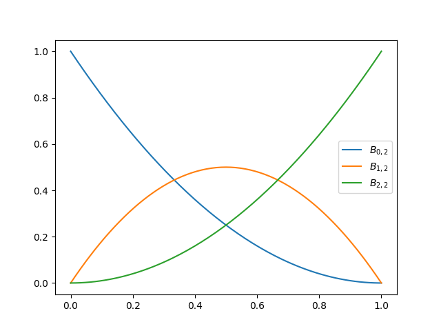
Bezier curves are the most simple type of NURBS, needing only the degree \(p\) to define the \((p+1)\) basis functions:

\[B_{i,p}(u) = \binom{p}{i}\left(1-u\right)^{p-i}\cdot u^{i}\]

At the interval \(u \in \left[0, \ 1\right]\) and \(\forall i=0, \ \cdots, \ p\)

Bezier curves can be described also by Splines, which uses the knotvector \(\textbf{U}\)

Degree 1

\[\mathbf{U} = \left[0, \ 0, \ 1, \ 1\right]\]

Degree \(p\)

\[\mathbf{U} = \left[\underbrace{0, \ \cdots, \ 0}_{p+1}, \ \underbrace{1, \ \cdots, \ 1}_{p+1}\right]\]

Use example

import numpy as np
from matplotlib import pyplot as plt
from pynurbs import GeneratorKnotVector, Function

degree = 2
knotvector = GeneratorKnotVector.bezier(degree)
bezier = Function(knotvector)

uplot = np.linspace(0, 1, 129)
for i in range(degree + 1):
    label = r"$B_{%d,%d}$" % (i, degree)
    plt.plot(uplot, bezier[i](uplot), label=label)
plt.legend()
plt.show()

Although above the function \(B_{i,p}(u)\) is described only by \(p\), bellow we have the graphs of the basis functions by using the knotvector. They are in svg format and therefore you can open and expand to see better the image.

B-Spline

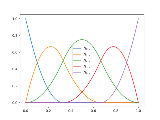
B-Splines uses the knotvector \(\mathbf{U}\) and is recursevelly defined by

\[\begin{split}N_{i,0}(u) = \begin{cases}1 \ \ \ \text{if} \ u_{i} \le u < u_{i+1} \\ 0 \ \ \ \text{else} \end{cases}\end{split}\]

\[N_{i,j}(u) = \dfrac{u - u_i}{u_{i+j}-u_{i}} \cdot N_{i,j-1}(u) + \dfrac{u_{i+j+1}-u}{u_{i+j+1}-u_{i+1}} \cdot N_{i+1,j-1}(u)\]

Use example

import numpy as np
from matplotlib import pyplot as plt
from pynurbs import GeneratorKnotVector, Function

degree, npts = 2, 5
knotvector = GeneratorKnotVector.uniform(degree, npts)
spline = Function(knotvector)

uplot = np.linspace(0, 1, 129)
for i in range(npts):
    label = r"$N_{%d,%d}$" % (i, degree)
    plt.plot(uplot, spline[i](uplot), label=label)
plt.legend()
plt.show()

BSpline Basis Functions of degree 2 and npts 5

Rational B-Spline

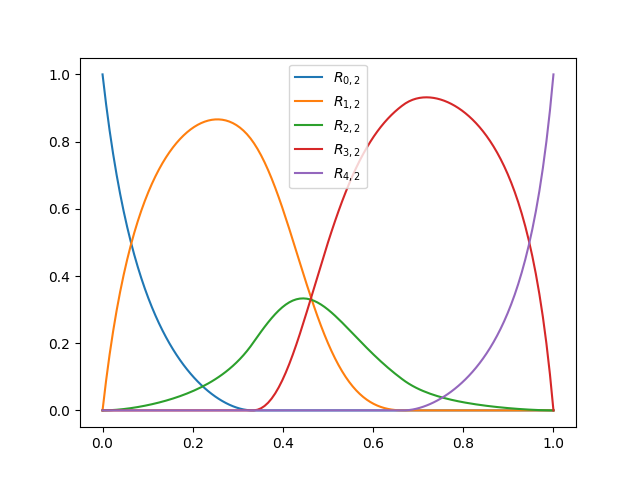
Like B-Splines, Rational B-Splines also uses the knotvector \(\mathbf{U}\), but along a weight vector \(\mathbf{w}\). It’s defined by

\[R_{i,j}(u) = \dfrac{w_{i} \cdot N_{i,j}(u)}{\sum_{k=0}^{n-1} w_{k} \cdot N_{k,j}(u)}\]

\[\mathbf{w} = \left[w_0, \ w_1, \ \cdots, \ w_{n-1}\right]\]

Use example

import numpy as np
from matplotlib import pyplot as plt
from pynurbs import GeneratorKnotVector, Function

degree, npts = 2, 5
knotvector = GeneratorKnotVector.uniform(degree, npts)
rational = Function(knotvector)
rational.weights = [1, 2, 0.5, 5, 2]

uplot = np.linspace(0, 1, 129)
for i in range(npts):
    label = r"$R_{%d,%d}$" % (i, degree)
    plt.plot(uplot, rational[i](uplot), label=label)
plt.legend()
plt.show()

Rational BSpline Basis Functions of degree 2 and 5 npts

Inserting knots in knotvector

We get an specific case and start inserting knots at center to see what happens with the basis functions

We start with the bezier of degree 3

\[\mathbf{U} = \left(0, \ 0, \ 0, \ 0, \ 1, \ 1, \ 1, \ 1 \right)\]

\[\mathbf{U} = \left(0, \ 0, \ 0, \ 0, \ 0.5, \ 1, \ 1, \ 1, \ 1 \right)\]

\[\mathbf{U} = \left(0, \ 0, \ 0, \ 0, \ 0.5,\ 0.5, \ 1, \ 1, \ 1, \ 1 \right)\]

\[\mathbf{U} = \left(0, \ 0, \ 0, \ 0, \ 0.5,\ 0.5, \ 0.5, \ 1, \ 1, \ 1, \ 1 \right)\]

\[\mathbf{U} = \left(0, \ 0, \ 0, \ 0, \ 0.5, \ 0.5,\ 0.5, \ 0.5, \ 1, \ 1, \ 1, \ 1 \right)\]

Non uniform splines

This section shows the basis function when the knotvector is not uniform.

We do it by inserting the knot \(0.25\) many times by starting with a bezier curve of degree 3

\[\mathbf{U} = \left(0, \ 0, \ 0, \ 0, \ 1, \ 1, \ 1, \ 1 \right)\]

\[\mathbf{U} = \left(0, \ 0, \ 0, \ 0, \ 0.25, \ 1, \ 1, \ 1, \ 1 \right)\]

\[\mathbf{U} = \left(0, \ 0, \ 0, \ 0, \ 0.25,\ 0.25, \ 1, \ 1, \ 1, \ 1 \right)\]

\[\mathbf{U} = \left(0, \ 0, \ 0, \ 0, \ 0.25,\ 0.25, \ 0.25, \ 1, \ 1, \ 1, \ 1 \right)\]

\[\mathbf{U} = \left(0, \ 0, \ 0, \ 0, \ 0.25, \ 0.25,\ 0.25, \ 0.25, \ 1, \ 1, \ 1, \ 1 \right)\]